Tutorial:
Camera time efficiency simulation

Content:

1. Introduction
2. Why I like these cameras
3. The Excel sheet with camera simulations: Low Dynamic, example 1
4. High Dynamic, example 2
5. Thermal Noise, example 3
6. High Dynamic and very weak signal, example 4
7. Readout Noise from calibration, example 5
8. Download of Excel sheet

3: The Excel sheet with camera simulations: Low Dynamic, example 1

Excel sheet:

The Excel sheet is very simple, but I have done some refinement lately. The goal with it is to get the time it take to have a final image with a given Signal to Noise ratio. These calculation are thought to have adapted telescopes that give equal photon flow per pixel for the different cameras because of different pixel sizes.

Here is an overview of the Excel sheet and first example:

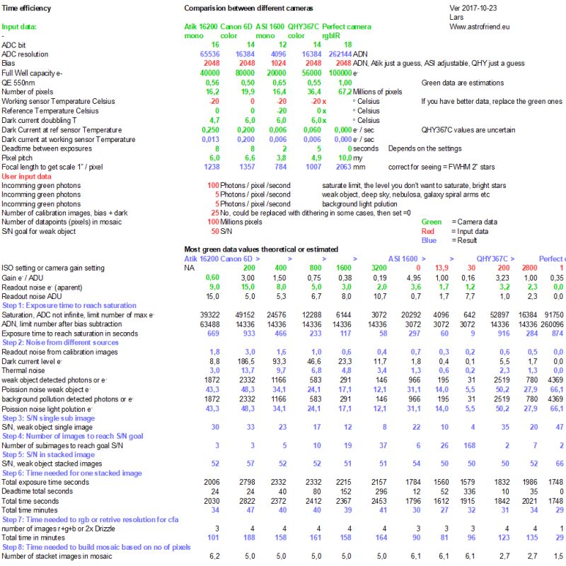
Data fields:

The green fields are the camera data, some examples:

• ADC, Analog Digital Converter's bit depth
• QE, cameras photon efficiency
• Full Well capacity, how many electrons a pixel can store, small pixels store less
• Dead time between photos, could be very important when doing Lucky Imaging
• Pixel pitch

It's not so easy to find the needed data, in some cases I just have estimated a value. You can replace them if you have a better idea of what it could be. Beware, behind the blue and green fields there are formulas, don't overwrite them!

Input fields:

Your input data are the red fields. Take a look at your old photos to have an idea what your telescope and camera delivers. Fitswork is easy to use for this purpose, use the CFA (before transform to color) if it's a color camera. Fitswork subtract the bias by automatic. Here I work only with the green pixels. If it's hard to recognize them do a linear interpolation deBayer with gain = 1 for all color to get a color image, examine interesting (saturate level, weak signals, background) green pixels in the center of images to not get any vignetting effects.

• Number of green wave length photons coming to one pixel per second
• The max flow of photons that you don't want to saturate, high levels keep the dynamic
• The weak flow of photons of the object you taken photos of
• The back ground photon flow from light pollution
• Your goal to what S/N ratio you want to have in the stacked image

The figures I have put in here are not to uncommon, but 100 incoming photons as max level before saturate is low and 5 photons per pixel and second is maybe high. It depends very much on the situation, object and telescope. Out of focus images give much lower peaks in level.

Output fields:

The output fields after calculation are blue.

It calculate which focal length that give a 1" / pixel scale for each camera and pixel pitch. It don't use this information but it could be interesting to know.

At lower half follow a list of steps with different calculated values:

• Step 1: Exposure time to reach saturation
• Step 2: Noise from different sources
• Step 3: S/N single sub image
• Step 4: Number of images to reach S/N goal
• Step 5: S/N in stacked image
• Step 6: Time needed for one stacked image
• Step 7: Time needed to rgb or retrive resolution for cfa
• Step 8: Time needed to build mosaic based on no of pixels

Step 1:
This is thought to be the highest level that you don't want to saturate. Too long exposure and you get low dynamic but less noise in the subs. You can take many short subs and stack them and then get better dynamics. To succeed with short exposures the camera must have low readout noise.

In this first example I have set highest signal that I don't want to saturate to 100 photons / pixel / seconds. Not very high but of course it depends on telescope or camera lens used. In most cases I will say this create a low contrast image with bright stars clipped.

Step 2:
As it's now it calculate noise from read out, dark current, object and light pollution. You can test with different signal flow from a weak object and different light pollution background. Analyze your old images, here is one method you can use: ../tutorial-find-photon-flow/tutorial-find-photon-flow.html. Light pollution noise can be high, but if you do narrow band imaging, like a H-Alpha filtered it's normally very low and then readout noise is more important to have low.

Step 3:
Here is the total Signal to Noise relation, S/N, calculated for one sub image. As you can see, a camera with small pixels has lower Full Well depth and get faster saturated, even worse with high gain. As a result you have to have shorter exposure time to not over saturate it. On the other hand with shorter exposure time you can take more of them.

Step 4:
In step 4 I do a calculation how many sub images it's needed to reach some S/N that you can set at the beginning. In this example S/N = 50. Heavy stretching of the image needs better quality. 50 could be a good value to start with. Number of images are rounded upwards. Compare the different cameras and the different settings of gain.

Step 5:
Here is the S/N ratio in the final stacked image, it differ a bit when number of images are low because of rounding error. They shall be close to the S/N value you set earlier.

Step 6:
Final we get how many minutes that is needed to make this image with different settings, it include the dead time between exposures.

Step 7:
This is an extra step. It gives information how much longer time it takes to make a color image from a mono chrome sensor, or how to recreate the lost resolution from a color camera with dithering technic ../tutorial-dithering/tutorial-dithering.html and Drizzle or similar method. See my other tutorials about Super Resolution with AIJ: ../tutorial-astroimagej-align-drizzle/tutorial-aij-align-introduction-matrix.html.

Step 8:
And last, it could be interesting to know how much longer it takes to built a mosaic from different cameras. If your interested in high resolution wide angle images this is important. In this case I refer to number of data points (pixels). It can be sensor area too. It calculates for seamless joints. Normally you have a overlap, but then you also get more exposure on the pixels, then less need of sub images. It gives about the same result when having S/N in mind.

As you see, the time difference differ a lot between cameras. But you should put in your own values that depends on your situation.

Test of different input values:

It can be very interesting to test with different input values. In this case the saturation level was adapted to a very low max signal and then low dynamic.

Note:
Even if a star is a point object in a normal telescope it spreads its photon not on only to one pixel, strong stars at least cover a radius of 3 pixels.

In next part I increased maximum level ten times to get better dynamics.